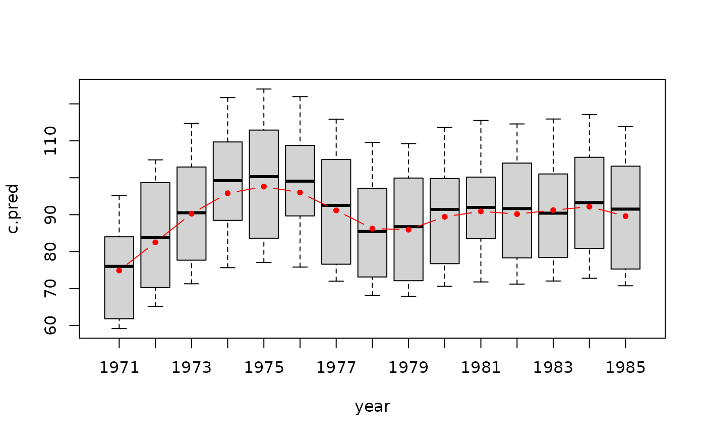
Fitting the temporal Metastatistical Extreme Value Distribution (TMEV)
ftmev.RdFit the temporal MEVD distribution TMEV to rainfall observations with a cyclic spline to account for seasonality.
Usage
ftmev(
  data,
  threshold = 0,
  minyears = 10,
  day_year_interaction = FALSE,
  verbose = FALSE,
  yday_ti_shape_k = 10,
  yday_ti_scale_k = 10,
  year_ti_shape_k = 10,
  year_ti_scale_k = 10
)
Arguments
- data
The data to which the TMEV should be fitted to.
datamust be a data.frame with two columns. The first column must contain dates of classDate, the second or last column must contain the rainfall values corresponding to datums in the rows. No negative values are allowed. NA values are removed with a warning.- threshold
A numeric that is used to define wet days as values > threshold. \(data <= threshold\) is set to NA.
- minyears
Minimum number of available years for fitting a cyclic spline to the non-stationary data series (see details).
- day_year_interaction
Logical. Should an additional year vs day of the year interaction be used for the calculation of the temporal trend in seasonality? (see details). Default is
FALSE.- verbose
Logical. If
TRUE, verbose output of the temporal fitting process is shown during runtime.- yday_ti_shape_k
A numeric that is used to set the dimension of the bases used to represent the smooth term ti() for yday in the formula for shape.
- yday_ti_scale_k
A numeric that is used to set the dimension of the bases used to represent the smooth term ti() for yday in the formula for scale.
- year_ti_shape_k
A numeric that is used to set the dimension of the bases used to represent the smooth term ti() for year in the formula for shape (only used when day_year_interaction == TRUE).
- year_ti_scale_k
A numeric that is used to set the dimension of the bases used to represent the smooth term ti() for year in the formula for scale (only used when day_year_interaction == TRUE).
Value
A list of class mevr with components:
- c
Vector of Weibull scale parameters of the TMEV, each row refers to one event, which is a day for daiyl rainfall.
- w
Vector of Weibull shape parameters of the TMEV, each row refers to one event, which is a day for daiyl rainfall.
- n
Number of wet events per year. Wet events are defined as rainfall >
threshold.- maxima
Maximum values corresponding to each year.
- data
A data frame with the data used to fit the TMEV and the fitted Weibull parameters
candw.- years
Vector of years as YYYY.
- threshold
The chosen threshold.
- x
The fitted
bamlssobject.- type
The type of distribution ("TMEV").
- minyears
The minimum number of years used to fit the TMEV as provided.
Details
With the aim of exploiting the full temporal information for parameter estimation, Falkensteiner et al., (2023) introduced the TMEV, which is an explicitly non-stationary formulation of the MEVD (Marani and Ignaccolo, 2015). Adopting a Weibull distribution for ordinary rainfall events, the assumption of yearly constant coefficients is relaxed by allowing the Weibull parameters to fluctuate with time. The TMEV can then be written as
$$F = \frac{1}{T} \sum_{j=1}^T \prod_{k \in A_j} \left( 1-e^{-\left(\frac{x}{C(j,k)}\right)^{w(j,k)}} \right)$$
with \(w > 0\) and \(C > 0\) being the Weibull shape and scale parameters, and $A_j \subseteq (1, ..., 366)$ being the wet days in year j. The temporal and the superimposed seasonal dependence on w and c is modeled with a cyclic seasonal effect on the day of the year.
Technically this is accomplished by fitting a cyclic spline to the daily rainfall
values. The following formula is used for the fitting procedure of both the Weibull scale and
shape parameter with the function bamlss from package bamlss:
$$parameter = x \sim s(year) + ti(yday, bs = "cc", k = 10)$$
The first effect models the long-term temporal trend of the parameter with a thin-plate spline.
The second effect models the superimposed seasonal fluctuations of the parameter
with the 'day of the year' with a cyclic cubic regression spline and 10 knots,
to ensure a smooth transition between December and January. The number of knots (k)
in the above equation can be set separately for the year and yday effect as well as
separately for the shape and scale parameter of the Weibull distribution. This can be done
by overwriting the parameters yday_ti_shape_k, yday_ti_scale_k,
year_ti_shape_k, year_ti_scale_k in the call to ftmev. Note that
these values depend on many factors, such as the structure of the data, the TMEV is fitted to.
Please refer to the documentation of the packages bamlss and,
in particular mgcv.
For data series with lengths < 10 years, the first temporal effect is changed to a simple linear time trend.
For trend analysis, an additional interaction term can be added to the model formula. The following term models the relationship between the seasonality as day of the year and the year itself with a combination of a thin plate and a cyclic cubic spline:
$$ti(year, yday, bs = c("tp", "cc"), d = c(1, 1), k = c(year_ti_k, yday_ti_k))$$
This function returns the parameters of the fitted TMEV distribution as well as some additional fitting results and input parameters useful for further analysis.
References
Marani, M. and Ignaccolo, M. (2015) 'A metastatistical approach to rainfall extremes', Advances in Water Resources. Elsevier Ltd, 79(Supplement C), pp. 121-126. doi: 10.1016/j.advwatres.2015.03.001.
Falkensteiner, M., Schellander, H., Hell, T. (2023) 'Accounting for seasonality in the metastatistical extreme value distribution', (Weather and Climate Extremes, 42, 2023, https://doi.org/10.1016/j.wace.2023.100601).

